Tutorials, Main Tools
This section is meant to help you familiarize yourself with the workflow of the main grsq tools.
The central hurdle is usually to make sure your RDF-data is correctly read in by grsq. This
might seem a bit cumbersome, but once you get the hang of it, it becomes really fast and easy
to test out all the various corrections, calculate scattering between sub-sets of RDFs, scan
damping parameters and so on. It’s worth it, promise!
For solute-solvent MD simulations, it is often useful to sub-partition all of your sampled pair-RDFs into whether:
Both atom types sampled are in the solute (the ‘solute’ term, giving the scattering \(I_{uu}(q)\))
Both atom types sampled are in the solvent (the ‘solvent’ term, \(I_{vv}(q)\))
One of the atom types is in the solute, and the other is in the solvent (the ‘cross’ terms \(I_{uv}(q)\) and \(I_{vu}(q)\))
Where the ‘atom type’ is defined as ‘an atom with the same form factor’ (often simply an element).
The total scattering signal is thus a sum of these terms:
If we look at the central equation that we need to evaluate to get to an x-ray scattering signal from a set of RDFs (i.e. the generalized Debye equation, see this paper for details):
where \(f_l(q)\) and \(f_m(q)\) are the atomic form factors, \(\delta_{w_lw_m}\) is the Kronecker delta, \(N_l\) and \(N_m\) are the numbers of atoms of type \(l\) and \(m\) respectively, \(g_{lm}(r)\) is the RDF beween atom types \(l\) and \(m\), and \(V\) is the volume of your MD simulation cell. \(g^0_{w_lw_m} = 0\) when \(w_l= u\) and \(w_m = u\), and 1 otherwise. Lastly, \(R\) is the \(r\)-distance at which you want to truncate your integral. The exact equation goes to infinity, but your sampled RDFs dont. By default, grsq will integrate until the end of your sampled RDFs. We will return to this in one of the tutorials.
Based on this, we can gather that the information you need to calculate the scattering from your set of RDFs is:
The g(r) sampled from your MD trajectory(/ies). This can be done efficiently with e.g. VMD, MDTraj, or MDAnalysis
The numbers of each atom type
The volume of your simulation cell
The atomic form factors are most often tabulated within the Independent Atom Model (IAM), which grsg uses the python package periodictable to retrieve. So unless you need to specifically modify them, you don’t need to think about getting those.
That’s it!
Note
GRSQ expects Å for lengths, Å-3 for volumes, and Å-1 for q-vectors.
Let’s start simple:
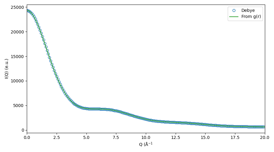
The Equivalence of The Discrete- and General Debye Equation
In this example, we manually enter the information we need to check that the
generalized Debye equation used on an RDF between two single atoms gives the
same as simply using the discrete Debye using the discrete distance between the
two atoms. grsq also includes various implementations of the discrete Debye
function, See the Tutorials, Supplementary Tools for more information.
from ase.io import read
from grsq.debye import Debye
from grsq.grsq import RDF
import numpy as np
import matplotlib.pyplot as plt
# Read in an xyz file of the two particles into an ASE object
atoms = read('data/tut1/2particle.xyz')
# Define Debye object with a qvector range
deb = Debye(qvec=np.arange(0, 20, 0.01))
# Calculate scattering
i_deb = deb.debye(atoms)
### Setup the RDF object for the two atoms:
# The xyz file contains to Pt atoms:
stoich = {'Pt_u':2}
# The RDF was sampled with VMD given a square box of 10 Å
V = 10**3
# Load the sampled RDF
rdf_dat = np.genfromtxt('data/tut1/gPt_u-Pt_u.dat')
# initialse the RDF object
rdf = RDF(rdf_dat[:, 0], # r, in Å
rdf_dat[:, 1], # g(r)
'Pt', 'Pt', # atom types: g_{Pt,Pt}(r)
'solute', 'solute', # atom region: this solute-only system
qvec=deb.qvec) # use the same q as for the debye
rdf.n1 = 2 # number of atoms
rdf.n2 = 2
rdf.volume = V # Volume of 'simulation cell'
iq = rdf.i_term1() # Calculate the atomic term
iq += rdf.i_term2() # Calculate the interatomic term
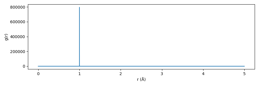
# plot the RDF, so we can see what it looks like.
fig, ax = plt.subplots(1, 1, figsize=(9, 3))
ax.plot(rdf_dat[:, 0 ], rdf_dat[:, 1])
ax.set_ylabel('g(r)')
ax.set_xlabel('r (Å)')
fig.tight_layout()
fig.savefig('gfx/tut1_gr.png')
# Plot the two ways of calculating I(Q) on top of each other
fig, ax = plt.subplots(1, 1, figsize=(9, 5))
ax.plot(deb.qvec[::10], i_deb[::10],
'C0o', label='Debye', mfc='None')
ax.plot(rdf.qvec, iq, 'C2-', label='From g(r)')
ax.set_xlim([0, 20])
ax.set_xlabel('Q (Å$^{-1}$')
ax.set_ylabel('I(Q) (e.u.)')
ax.legend(loc='best')
fig.tight_layout()
fig.savefig('gfx/tut1_iq.png')
This was perhaps an excessive amount of manual work - but you don’t need to. This only serves the purpose of looking a bit under the hood to see what’s going on.
Using RDFSets
The same \(I_{uu}(Q)\) can be obtained much more quickly:
import numpy as np
import matplotlib.pyplot as plt
from grsq.grsq import rdfset_from_dir

# Use the helper function to read in the RDF(s)
rdfs = rdfset_from_dir('data/tut1/',
                       volume=10**3,
                       stoich={'Pt_u':2})
iq = rdfs.get_iq(qvec=np.arange(0, 20, 0.01))

# Plot
fig, ax = plt.subplots(1, 1, figsize=(9, 5))
# this time we just use the r vector from the first
# - and only - rdf in the set
ax.plot(rdfs[0].qvec,  iq, 'C2-', label='From g(r)')
ax.set_xlim([0, 20])
ax.set_xlabel('Q (Å$^{-1}$')
ax.set_ylabel('I(Q) (e.u.)')
ax.legend(loc='best')
fig.tight_layout()
fig.savefig('gfx/tut1_iq_simple.png')
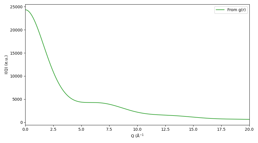
Here, we’ve used the helper function grsq.grsq.rdfset_from_dir()
to load all the rdf data files from a subdirectory - in this case there is only
one. This requires that the files have a certain name-format, check its docstring
for details.
Really Using RDFSets
An RDFSet is an OrderedDict with some extra functionalities. You can apply finite-size corrections across all (solvent-solvent and solute-solvent) RDFs, calculate the X-ray scattering terms:
Total signal (as in the previous tutorial):
rdfs.get_iq(qvec)Solute-Solvent (cross):
rdfs.get_cross(qvec)Solvent-Solvent:
rdfs.get_solvent(qvec)Displaced (Excluded) Volume:
rdfs.get_dv(qvec)
Define subsets of RDFs to analyse further, and add RDFSets together
as you do python lists.
To test this out, we need some more RDFs. The gitlab repo of grsq contains some we can use, in the data/rdfsets directory here
Since you can have formatted your RDF files in a myriad of ways yourself, we refrain from using the helper function from before, and simply write a small piece of code that makes the RDFSet from scratch:
import glob
import numpy as np
from grsq.grsq import RDF, RDFSet

# Data files are named 'u' for solUte, 'v' for solVent
t = {'u':'solute', 'v':'solvent'}

# Stoichometry from the MD simulation:
stoich = {'u': {'Fe':1, 'C':30, 'N':6, 'H':24},
          'v': {'O':7329, 'H':14682}}
# Volume from the MD simulation:
vol = 277088.4332

# List all data files, change the path to where you put them:
data_files = sorted(glob.glob('data/rdfsets/*dat'))

rdfs = RDFSet()
for df in data_files:
    data = np.genfromtxt(df)  # load the data file
    # Get r and g(r), in this case they're in these columns:
    r = data[:, 0]
    g = data[:, 1]
    # Get the element and region from the file names
    # this can be a bit cumbersome, depending on
    # how you have stored this information
    file_name = df.split('/')[-1]
    el1 = file_name.split('g')[1].split('_')[0]
    re1 = file_name.split('_')[1].split('-')[0]
    el2 = file_name.split('-')[1].split('_')[0]
    re2 = file_name.split('_')[2].split('.')[0]

    # Create RDF object
    rdf = RDF(r=r, g=g, name1=el1, name2=el2,
              region1=t[re1], region2=t[re2],
              n1=stoich[re1][el1], n2=stoich[re2][el2],
              volume=vol)
    # Add g_AB to RDFSet ...
    rdfs.add_rdf(rdf)
    # .. And also g_BA:
    rdfs.add_flipped(rdf)
Note that we are manually adding g_BA(r) from the g_AB(r) data. The directory only contained g_AB(r) datafiles and not also g_BA(r), since they are identical, and it thus makes no sense to sample both of them. However, the RDFSet still needs both to get the right amplitude of the individual signals in the end. See our paper for details.
Now, you should have the following:
rdfs.show():

|  #  | KEY                     |     STOICHOMETRY     | REGION1, REGION2 | VOLUME
| 000 | C-solute--C-solute      | N1:    30, N2:    30 | solute , solute  | 277088.4332 |
| 001 | C-solute--Fe-solute     | N1:    30, N2:     1 | solute , solute  | 277088.4332 |
| 002 | Fe-solute--C-solute     | N1:     1, N2:    30 | solute , solute  | 277088.4332 |
| 003 | C-solute--H-solute      | N1:    30, N2:    24 | solute , solute  | 277088.4332 |
| 004 | H-solute--C-solute      | N1:    24, N2:    30 | solute , solute  | 277088.4332 |
| 005 | C-solute--H-solvent     | N1:    30, N2: 14682 | solute , solvent | 277088.4332 |
| 006 | H-solvent--C-solute     | N1: 14682, N2:    30 | solvent, solute  | 277088.4332 |
| 007 | C-solute--N-solute      | N1:    30, N2:     6 | solute , solute  | 277088.4332 |
| 008 | N-solute--C-solute      | N1:     6, N2:    30 | solute , solute  | 277088.4332 |
| 009 | C-solute--O-solvent     | N1:    30, N2:  7329 | solute , solvent | 277088.4332 |
| 010 | O-solvent--C-solute     | N1:  7329, N2:    30 | solvent, solute  | 277088.4332 |
| 011 | Fe-solute--H-solute     | N1:     1, N2:    24 | solute , solute  | 277088.4332 |
| 012 | H-solute--Fe-solute     | N1:    24, N2:     1 | solute , solute  | 277088.4332 |
| 013 | Fe-solute--H-solvent    | N1:     1, N2: 14682 | solute , solvent | 277088.4332 |
| 014 | H-solvent--Fe-solute    | N1: 14682, N2:     1 | solvent, solute  | 277088.4332 |
| 015 | Fe-solute--N-solute     | N1:     1, N2:     6 | solute , solute  | 277088.4332 |
| 016 | N-solute--Fe-solute     | N1:     6, N2:     1 | solute , solute  | 277088.4332 |
| 017 | Fe-solute--O-solvent    | N1:     1, N2:  7329 | solute , solvent | 277088.4332 |
| 018 | O-solvent--Fe-solute    | N1:  7329, N2:     1 | solvent, solute  | 277088.4332 |
| 019 | H-solute--H-solute      | N1:    24, N2:    24 | solute , solute  | 277088.4332 |
| 020 | H-solute--H-solvent     | N1:    24, N2: 14682 | solute , solvent | 277088.4332 |
| 021 | H-solvent--H-solute     | N1: 14682, N2:    24 | solvent, solute  | 277088.4332 |
| 022 | H-solute--N-solute      | N1:    24, N2:     6 | solute , solute  | 277088.4332 |
| 023 | N-solute--H-solute      | N1:     6, N2:    24 | solute , solute  | 277088.4332 |
| 024 | H-solute--O-solvent     | N1:    24, N2:  7329 | solute , solvent | 277088.4332 |
| 025 | O-solvent--H-solute     | N1:  7329, N2:    24 | solvent, solute  | 277088.4332 |
| 026 | H-solvent--H-solvent    | N1: 14682, N2: 14682 | solvent, solvent | 277088.4332 |
| 027 | N-solute--H-solvent     | N1:     6, N2: 14682 | solute , solvent | 277088.4332 |
| 028 | H-solvent--N-solute     | N1: 14682, N2:     6 | solvent, solute  | 277088.4332 |
| 029 | N-solute--N-solute      | N1:     6, N2:     6 | solute , solute  | 277088.4332 |
| 030 | N-solute--O-solvent     | N1:     6, N2:  7329 | solute , solvent | 277088.4332 |
| 031 | O-solvent--N-solute     | N1:  7329, N2:     6 | solvent, solute  | 277088.4332 |
| 032 | O-solvent--H-solvent    | N1:  7329, N2: 14682 | solvent, solvent | 277088.4332 |
| 033 | H-solvent--O-solvent    | N1: 14682, N2:  7329 | solvent, solvent | 277088.4332 |
| 034 | O-solvent--O-solvent    | N1:  7329, N2:  7329 | solvent, solvent | 277088.4332 |
That looks correct. We can quickly check how many combinations we should have:
import itertools
atom_types = [f'{atom}-{region}'
            for region, elements in stoich.items()
            for atom in elements]
len(list(itertools.product(atom_types, repeat=2)))

>>> 36
We only have 35, but there is also only one Fe atom, so there is no Fe-Fe RDFs. That adds up!
Now we can apply low-q corrections (see the next tutorial), damping windows, and simulate the X-ray scattering signal:
import matplotlib.pyplot as plt
from grsq.damping import Damping
# Applies van der Vegt correction to all relevant RDFs.
# This overwrites the g(r) values with the corrected values
# So if you do it twice, you have overcorrected!
rdfs.vdv_correct()
# Init a Lorch damping object with L = 1/2 box (to which the RDFs are sampled)
damp = Damping('lorch', L=rdfs[0].r[-1])
# Define a q vector
qvec = np.arange(0, 6, 0.01)
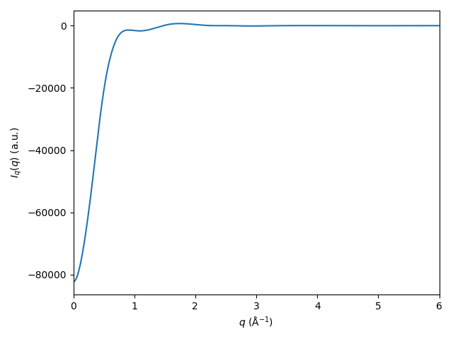
# Calculate the cross term (for example):
I_c = rdfs.get_cross(qvec=qvec, damping=damp)
plt.plot(qvec, I_c)
plt.xlim([0, 6])
plt.xlabel('$q$ (Å$^{-1}$)')
plt.ylabel('$I_c(q)$ (a.u.)')
plt.tight_layout()
plt.show()
Try yourself to calculate and plot the solute term, the solvent term, and the displaced-volume term.
Sub-selections
With the rdfs in hand, you can quickly analyse subsets of various pairs you want to investigate the
scattering from, to get an overview of which pairs contribute what to the total signal(s).
An example:
# Fe-Solvent only
fe_solv = RDFSet()
for key, rdf in rdfs.items():
# Find whichever RDFs you're interested in, for example:
if (('Fe' in key[0]) and (rdf.region2 =='solvent')):
fe_solv[key] = rdf
fe_solv.add_flipped(rdf)
fe_solv.show()
# N-Solvent only
n_solv = RDFSet()
for key, rdf in rdfs.items():
# Find whichever RDFs you're interested in, for example:
if (('N' in key[0]) and (rdf.region2 =='solvent')):
n_solv[key] = rdf
n_solv.add_flipped(rdf)
n_solv.show()
# You can also add RDFSets:
combined = fe_solv + n_solv
I_combined = combined.get_cross(qvec=qvec, damping=damp)
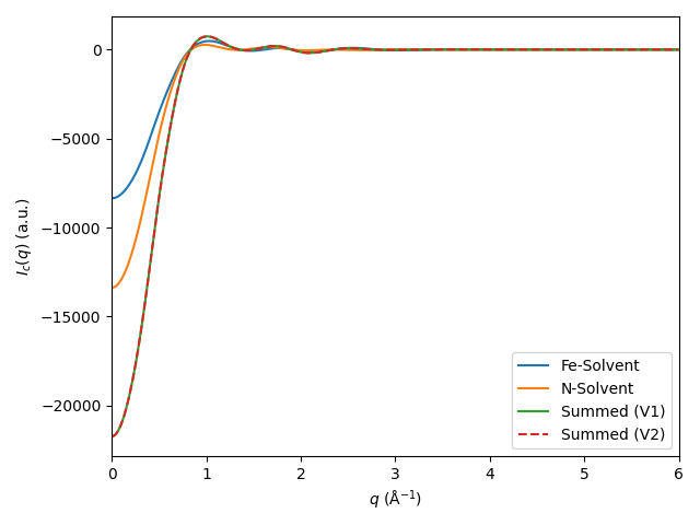
I_fe_solv = fe_solv.get_cross(qvec=qvec, damping=damp)
I_n_solv = n_solv.get_cross(qvec=qvec, damping=damp)
plt.plot(qvec, I_fe_solv, label='Fe-Solvent')
plt.plot(qvec, I_n_solv, label='N-Solvent')
plt.plot(qvec, I_n_solv + I_fe_solv, label='Summed (V1)')
plt.plot(qvec, I_combined, '--', label='Summed (V2)')
plt.xlim([0, 6])
plt.legend(loc='best')
plt.xlabel('$q$ (Å$^{-1}$)')
plt.ylabel('$I_c(q)$ (a.u.)')
plt.tight_layout()
plt.show()
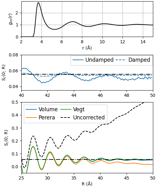
Using and analysing finite-size corrections
As described in detail in our paper, a useful method for checking how well your chosen finite-size correction performed is to calculate the structure factor from a corrected RDF at \(q=0\) Å \(^{-1}\) at increasing truncation-lengths \(R\) of the integral in the generalized Debye equation.
To illustrate this, let us recreate Fig. 3(B) in the paper.
import copy
import numpy as np
import matplotlib.pyplot as plt
from grsq.grsq import RDF
from grsq.damping import Damping

V = 100**3  # Volume of the simulation cell

data = np.genfromtxt('data/tut3/tut_gAr_v-Ar_v.dat')

# Only calculate S(q=0)
qvec = np.array([0])

# There is only a single RDF, so we don't need the RDFSet class here..
rdf_raw = RDF(r=data[:, 0], g=data[:, 1],
              name1='Ar', name2='Ar',
              region1='solvent', region2='solvent',
              n1=20712, n2=20712,
              volume=V, qvec=qvec)

# find the first nonzero g(r) r value
r_first_nonzero = rdf_raw.r[np.where(rdf_raw.g > 0)[0]][0]

# Fitted volume correction: Fit from r > 41 Å
opt = rdf_raw.fit(r_first_nonzero, fit_start=41, fit_stop=rdf_raw.r[-1])

# Prepare to loop through all 3 corrections
corrections = ('volume', 'perera', 'vegt')
corr_vars = ({'Ri':opt.x[0]},  # use the fitted value
             {'Ri':r_first_nonzero, # as prescribed in
              'R_avg':35},   # Perera et al
             {}) # van der Vegt is parameterless

# Define R truncation values for S(0; R)
rmaxs = np.arange(0.0001, 50, 0.1)

# Define function to get S(0; R)
def get_s0(rdf, damp=None):
    s = np.zeros((len(qvec), len(rmaxs)))
    for j, r_max in enumerate(rmaxs):
        rdf.qvec = qvec
        rdf.damp = damp
        rdf.r_max = r_max
        s[:, j] = rdf.structure_factor()
    return s

# Set up the figure
fig = plt.figure(constrained_layout=True, figsize=(5, 6))
gs1 = fig.add_gridspec(nrows=4, ncols=1, left=0.05, right=0.48, hspace=0)
ax0 = fig.add_subplot(gs1[0])
ax2 = fig.add_subplot(gs1[1])
ax1 = fig.add_subplot(gs1[2:])

# Apply the corrections, and plot them
avgs = []
for c, corr in enumerate(corrections):
    # copy the uncorrected rdf object
    rdf_cor = copy.deepcopy(rdf_raw)
    # apply correction
    rdf_cor.g = rdf_cor.correct(method=corr, **(corr_vars[c]))
    # get S(0; R)
    s0 = get_s0(rdf_cor, damp=None)
    ax1.plot(rmaxs, s0[0], label=corr.title())
    # Save the converged value
    avgs.append(np.mean(s0[0][rmaxs > 40]))

# plot the converged value of the Vegt correction
ax1.axhline(avgs[-1], color='k', ls='-.')
# plot the raw RDF
ax1.plot(rmaxs, get_s0(rdf_raw)[0], 'k--', label='Uncorrected')
# polish plot
ax1.legend(loc='best', fontsize=12,
           ncol=2, columnspacing=0.5,
           handletextpad=0.4)
ax1.set_xlabel('R (Å)')
ax1.set_ylabel('$S_c$(0; R)')
ax1.set_xlim([25, 50])
ax1.set_ylim([-.05, 0.5])

# Plot the RDF
ax0.plot(rdf_raw.r, rdf_raw.g, 'k')
ax0.set_xlabel('r (Å)')
ax0.set_ylabel('$g_{lm}$(r)')
ax0.set_yticks([0, 1, 2])
ax0.set_ylim([0, 2.95]);
ax0.set_xlim([2, 15]);
ax0.grid()

### Middle plot: Compare damped and undamped
# Using the Lorch damping window

## First plot the corrected, undamped
rdf_cor = copy.deepcopy(rdf_raw)
rdf_cor.g = rdf_cor.correct(method='volume', Ri=opt.x[0])
s0 = get_s0(rdf_cor, damp=None)
ax2.plot(rmaxs, s0[0], label='Undamped')

## Then plot the corrected, damped
# init damping object
damp = Damping('lorch', L=rdf_cor.r[-1])
# correct, damp, get_s0, plot:
rdf_cor = copy.deepcopy(rdf_raw)
rdf_cor.g = rdf_cor.correct(method='volume', Ri=opt.x[0])
s0 = get_s0(rdf_cor, damp=damp)
ax2.axhline(avgs[-1], color='k', ls='-.', zorder=30)
ax2.plot(rmaxs, s0[0], 'C0--', label='Damped')
ax2.set_xlim([40, 50])
ax2.set_ylim([0.035, 0.08])
ax2.legend(loc='upper right', fontsize=12,
           ncol=2, columnspacing=0.35,
           handletextpad=0.4,
           borderaxespad=0.1)
ax2.set_ylabel('$S_c$(0; R)')
fig.savefig('gfx/tut3.png')