Tutorials, Supplementary Tools
The Discrete Debye Equation for ASE Atoms Objects
While ASE has its own implementation of the Debye equation, the grsq
implementation has a slightly different set of functionalities, as well
as a two that speeds up the calculation for large atomic systems like clusters,
nanoparticles, slabs, etc … :
A Numba-based parallel implementation
A simple histogram-approximation to the discrete Debye Equation
The numba implementation gives the exact same result as the pure python implementation (within numerical accuracies), while the accuracy of the histogram histogram-approximation decreases with the size of the bins of the histogram.
The plot below compares the computation time (on a 2021 M1 Max MacBook Pro) of the pure python implementation with the two other methods:
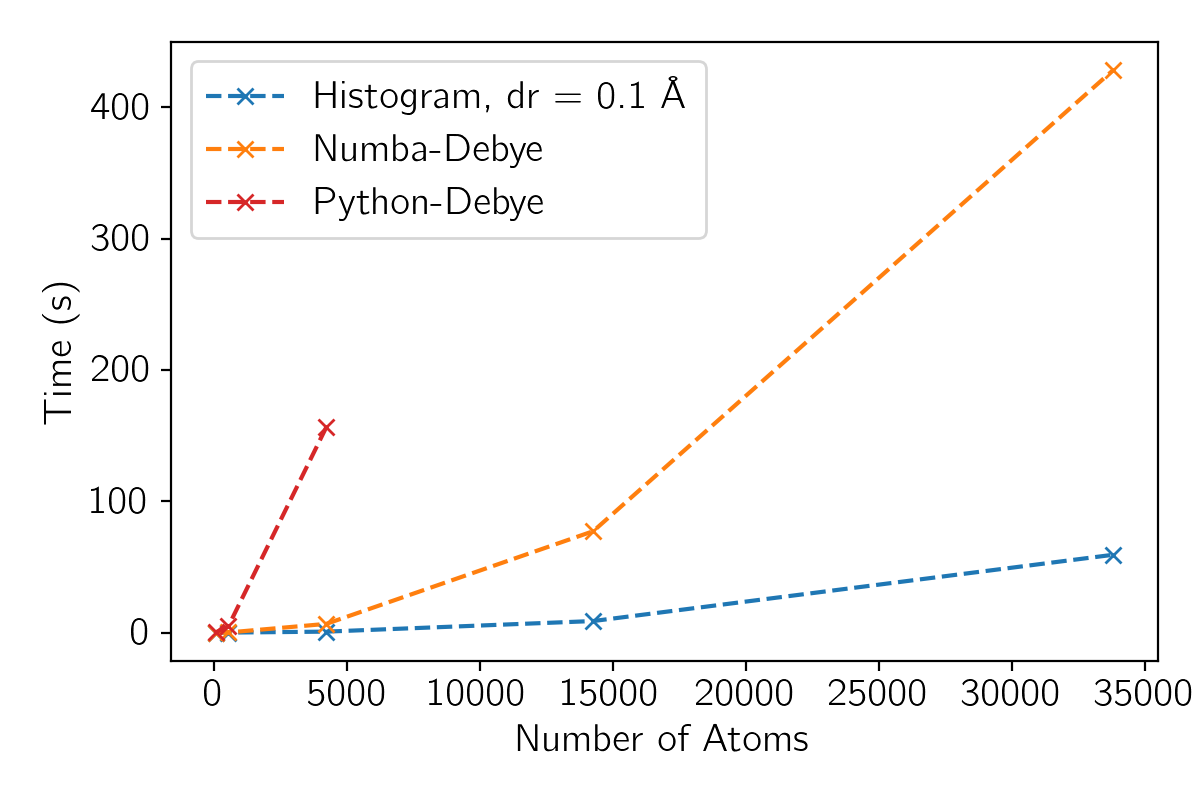
The histogram method scales very nicely, but be sure to check that your chosen bin size provides acceptable accuracy for the signal you want to simulate.
Note
The grsq Debye code uses periodictable to retrieve the
atomic form factors, based on the Cromer-Mann parametrization, using
the Waasmeier & Kirfel parameters. As
default, it takes the parameters for the the electrically neutral
element of each ASE Atom. You can also enter custom form factors,
if required. Please refer to the Using custom atomic form factors
section for more information on custom atomic form factors.
Debye and Debye-Numba
Calculating the scattering with either of these two methods is
straightforward, here shown using a molecule xyz from the grsq tests
import numpy as np
from grsq.debye import Debye
from ase.io import read  # for example

qvec = np.arange(0, 7, 0.01)
deb = Debye(qvec=qvec)
atoms = read('tests/data/testmol.xyz')

i_slow = deb.debye(atoms)  # use the pure-python method
i_fast = deb.debye_numba(atoms)  # use the numba-accelerated method

fig, ax = plt.subplots(1, 1, figsize=(6, 4))
ax.plot(deb.qvec, i_slow, label='Debye, Python')
ax.plot(deb.qvec, i_fast, '--', label='Debye, Numba')
ax.set_xlim([0, 7])
ax.set_xlabel('q (Å$^{-1}$)')
ax.set_ylabel('I(q) (a.u.)')
ax.legend(loc='best')
fig.tight_layout()

The Histogram Approximation
See e.g. this paper for details.
In the same manner as for the RDF-based Debye expression (which is basically just a differently normalized histogram), we can split up the terms by ‘atom type’, i.e. atoms that scatter in the same way. For the atoms of type \(l\) and \(m\), all \(i\) form factors are the same, as is all \(j\):
and then approximate the discrete distances with a histogram \(n_{lm}(r_k)\) of all distances between \(l\) and \(m\)-type atoms:
The total scattering signal is then obtained by summing over all possible combinations of atom types:
where \(\delta_{lm}\) is the Kronecker delta, ensuring that only the upper triangular terms in the double sum are evaluated, since \(n_{lm}(r_k) = n_{ml}(r_k)\) and thus \(I_{lm}(q) = I_{ml}(q)\).
The following code-snippet compares the X-ray signal calculated from the discrete debye formulation to the histrogrammed approximation for a series of increasing bin sizes:
import time
import numpy as np
import matplotlib.pyplot as plt
from ase.spacegroup import crystal
from grsq.debye import Debye

### Create heteroatomic nanoparticle for testing
a = b = 2.81
c = 13.91
lico2 = crystal(['Li', 'Co', 'O'],
                basis=[(0, 0, 0),
                    (1/3, 2/3, 1/6),
                    (0, 0, 0.24)],
                spacegroup='R-3m',
                cellpar=[a, b, c, 90, 90, 120])
lico2_chunk = lico2 * (20, 20, 10)
center = lico2_chunk.get_center_of_mass()
np_radius = 5 # 0.5 nm np
atoms = Atoms(cell=lico2_chunk.get_cell(), pbc=False)
for atom in lico2_chunk:
    if np.linalg.norm(atom.position - center) <= np_radius:
        atoms += atom

### Init Debye()
qvec = np.arange(0, 5, 0.01)
deb = Debye(qvec=qvec)
i_full = deb.debye_numba(atoms)

### Calculate the histogrammed approximation for a range of dr values
drs = [0.5, 0.2, 0.1, 0.05, 0.005, 0.001]
i_vsdr = np.zeros((len(qvec), len(drs)))
for j, dr in enumerate(drs):
    start = time.time()
    i_hist = deb.debye_histogrammed(atoms, dr=dr)
    end = time.time()
    i_vsdr[:, j] = i_hist

    diff = np.sum(np.abs(i_full - i_hist))
    pct_off = 100 * diff / i_full[0]

    print(f'dr: {dr:5.4f} Å, time: {(end - start) * 1e3:6.2f} ms, error: {pct_off:4.2f}%')


### Plot
cmap = plt.cm.viridis_r
colors = cmap(np.linspace(0, 1, len(drs)))
fig, ax = plt.subplots(1, 1, figsize=(6, 4))
ax.plot(deb.qvec[::10], i_full[::10], 'ko', mfc='none', label='Discrete Debye')
for j, dr in enumerate(drs):
    ax.plot(deb.qvec, i_vsdr[:, j], '-', color=colors[j], label=f'dr = {dr} Å')
ax.set_xlim([0.5, 5])
ax.set_ylim([0, .3e5])
ax.set_xlabel('q (Å$^{-1}$)')
ax.set_ylabel('I(q) (a.u.)')
ax.legend(loc='best', ncol=2)
fig.tight_layout()
Which produces:
dr: 0.5000 Å, time:   1.43 ms, error: 109.01%
dr: 0.2000 Å, time:   2.10 ms, error: 70.27%
dr: 0.1000 Å, time:   2.83 ms, error: 31.01%
dr: 0.0500 Å, time:   4.40 ms, error: 12.19%
dr: 0.0050 Å, time:  44.10 ms, error: 0.73%
dr: 0.0010 Å, time: 229.02 ms, error: 0.15%

Note
Periodic boundary conditions have not yet been implemented for the discrete debye or the histogram approximation, please use the g(r) -> I(q) method for periodic calculations.
Using custom atomic form factors
If you want to use a different form factor for an element, you can do so by initializing the Debye object with a dictionary:
from ase import Atoms
import numpy as np
from grsq.debye import Debye

# Enter your own Cromer-Mann Parameters in a dict:
cm = {'Pt': {'a': np.array([27.00590, 17.76390, 15.71310, 5.783700]),
            'b': np.array([1.512930, 8.811740, 0.4245930, 38.61030]),
            'c': 11.68830}}
deb = Debye(custom_cm=cm)
atoms = Atoms('Pt2', positions=[[0, 0, 0], [0, 0, 3]])
i_custom = deb.debye(atoms)
This overwrites the form factor for all of the atoms of this element in the ASE atoms object.
If you have an atomic system with two distinct atom types of the same element
- for example Mg and Mg2+ which has different atomic form factors within the
Cromer-Mann parametrization, you can pass in a list of custom elements, and
the code will read that instead of the symbols saved in the Atoms object:
# create unphysical Mg - Mg2+ system to show how custom_elements is used
atoms = Atoms('Mg2', positions=[[0, 0, 0], [0, 0, 3]])

# The CM parameters from https://www.classe.cornell.edu/~dms79/x-rays/f0_CromerMann.txt
cm = {'Mg2+': { 'a' : np.array([5.420400, 2.173500, 1.226900, 2.307300]),
                'b': np.array([2.827500, 79.26110, 0.3808000, 7.193700]),
                'c': 0.8584000},
      'Mg':   { 'a': np.array([3.498800, 3.837800, 1.328400, 0.8497000]),
                'b': np.array([2.167600, 4.754200, 0.1850000, 10.14110]),
                'c': 0.4853000}}

deb_ccm = Debye(custom_cm=cm)
i = deb_ccm.debye(atoms, custom_elements=['Mg2+', 'Mg'])
Compton Scattering Calculator
Parametrized as described in the paper by Haidu et al.
Currently only has parameters for the elements in this file, as well as for Tl, Pt and water.
To calculate the Compton scattering signal for a system that includes water, you have to input the element:count stoichometry as a dict:
import numpy as np
from grsq.compton import compton_scattering

qvec = np.arange(0, 7, 0.01)
atoms = {'C': 4, 'H2O': 256}
I = compton_scattering(atoms, qvec)
If you have system without water, you can also just input an ASE atoms object:
import numpy as np
from ase import Atoms
from grsq.compton import compton_scattering

qvec = np.arange(0, 7, 0.01)
atoms = Atoms('C4')
I = compton_scattering(atoms, qvec)